Week 3: General(ized) linear models
PLS 206 — the code behind the lectures
One page for the whole week. It follows the slides (Week3_GLM.pptx) in order, and has the code behind every figure and number in the lecture, with the output underneath.
To run it yourself, download either version and open it in RStudio. It reads the data straight from the course website, so there is no file to download and no working directory to set:
- Week3_GLM.R: the plain script. Each block is tagged
[CORE],[HANDY], or[DEMO]in a comment. - Week3_GLM.qmd: this page as a Quarto notebook (open in RStudio, run chunk by chunk, or click Render).
Every block of code on this page carries one of three labels:
- Core The analysis. Code you would run on your own data: fit the model, read the output, check the diagnostics, report it. Start here for the problem sets.
- Handy Useful, not essential. Wrangling, plotting, and small helpers that make the core easier. Worth knowing; skip on a first read.
- Demo For the lecture only. Simulated data, sums done by hand, and the code behind slide figures. It shows why the core works. Folded: click to open.
# install.packages(c("ggplot2", "emmeans", "car"))
library(ggplot2)
Part A. Groups as predictors
1) The data: a wheat field trial
90 plots: three varieties (Amber, Bronze, Copper) x two water treatments (control, drought), 15 plots of each, and a nitrogen rate (kg N/ha) that varies from plot to plot. Three responses: yield (t/ha), rust (stripe rust seen on the plot: 1 = yes, 0 = no), and aphids (aphids counted on 10 tillers). Simulated.
trial <- read.csv("https://greymonroe.github.io/PLS_206/data/wheat_trial.csv")
head(trial)
plot variety water nitrogen yield rust aphids
1 1 Copper control 19 2.32 0 0
2 2 Amber control 34 3.44 0 8
3 3 Bronze control 180 7.10 1 12
4 4 Bronze drought 63 2.51 0 1
5 5 Bronze control 117 5.51 1 30
6 6 Copper control 14 2.73 0 4table(trial$variety, trial$water) # check the design: 15 plots per combination
         control drought
  Amber       15      15
  Bronze      15      15
  Copper      15      15
# groups: violin + box + points
ggplot(trial, aes(water, yield, fill = water, colour = water)) +
geom_violin(alpha = 0.25, colour = NA) +
geom_boxplot(width = 0.18, fill = "white", colour = "grey30", outlier.shape = NA) +
geom_jitter(width = 0.08, height = 0) +
labs(x = NULL, y = "Yield (t/ha)") +
theme_classic() + theme(legend.position = "none")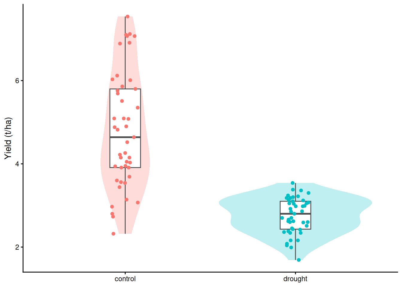
2) Two groups: a dummy variable
A group becomes a 0/1 column: 0 for control, 1 for drought. The intercept is the control mean; the coefficient is drought minus control.
m_water <- lm(yield ~ water, data = trial)
round(coef(summary(m_water)), 3)
Estimate Std. Error t value Pr(>|t|)
(Intercept) 4.806 0.152 31.523 0
waterdrought -2.051 0.216 -9.513 0tapply(trial$yield, trial$water, mean) # the two means control drought
4.806222 2.755111 Demo: the drought mean from the coefficients
coef(m_water)[1] + coef(m_water)[2] # intercept + difference = drought mean(Intercept)
2.755111 3) It’s a t-test
t.test(yield ~ water, data = trial, var.equal = TRUE) # same t and p as waterdrought
    Two Sample t-test

data:  yield by water
t = 9.5125, df = 88, p-value = 3.613e-15
alternative hypothesis: true difference in means between group control and group drought is not equal to 0
95 percent confidence interval:
 1.622607 2.479615
sample estimates:
mean in group control mean in group drought
             4.806222              2.755111
4) Under the hood: the design matrix
head(trial$water)[1] "control" "control" "control" "drought" "control" "control"head(model.matrix(m_water)) # the 0/1 column R made for you (Intercept) waterdrought
1 1 0
2 1 0
3 1 0
4 1 1
5 1 0
6 1 05) Which group is the intercept?
Text columns go in alphabetical order; the first level is the reference.
trial2 <- trial
trial2$water <- factor(trial2$water,
                       levels = c("drought", "control"))
coef(lm(yield ~ water, data = trial2))   # same model, flipped sign
(Intercept) watercontrol
2.755111 2.051111 Part B. More than two groups (ANOVA)
6) Three varieties, two dummies
The 45 control plots only, for now.
control <- subset(trial, water == "control")
tapply(control$yield, control$variety, mean)
Amber Bronze Copper
4.767333 6.156000 3.495333 m_var <- lm(yield ~ variety, data = control)
round(coef(summary(m_var)), 3) # each row: that variety minus Amber Estimate Std. Error t value Pr(>|t|)
(Intercept) 4.767 0.221 21.575 0
varietyBronze 1.389 0.312 4.444 0
varietyCopper -1.272 0.312 -4.070 0Demo: the design matrix with three groups
mm <- model.matrix(m_var)
head(cbind(control["variety"], mm), 7)   # Amber plots: zeros in both dummies
variety (Intercept) varietyBronze varietyCopper
1 Copper 1 0 1
2 Amber 1 0 0
3 Bronze 1 1 0
5 Bronze 1 1 0
6 Copper 1 0 1
8 Copper 1 0 1
12 Bronze 1 1 07) Do the varieties differ at all? One F-test
anova(m_var) # the one-way ANOVAAnalysis of Variance Table
Response: yield
Df Sum Sq Mean Sq F value Pr(>F)
variety 2 53.128 26.5638 36.269 7.085e-10 ***
Residuals 42 30.762 0.7324
---
Signif. codes: 0 '***' 0.001 '**' 0.01 '*' 0.05 '.' 0.1 ' ' 1summary(aov(yield ~ variety, data = control)) # the same table, Week 1 style Df Sum Sq Mean Sq F value Pr(>F)
variety 2 53.13 26.564 36.27 7.09e-10 ***
Residuals 42 30.76 0.732
---
Signif. codes: 0 '***' 0.001 '**' 0.01 '*' 0.05 '.' 0.1 ' ' 18) Which pairs? Tukey, and adjusting for many tests
TukeyHSD(aov(m_var)) Tukey multiple comparisons of means
95% family-wise confidence level
Fit: aov(formula = m_var)
$variety
diff lwr upr p adj
Bronze-Amber 1.388667 0.629451 2.1478823 0.0001841
Copper-Amber -1.272000 -2.031216 -0.5127843 0.0005836
Copper-Bronze -2.660667 -3.419882 -1.9014510 0.0000000# raw vs adjusted p-values for every pair
pairwise.t.test(control$yield, control$variety, p.adjust.method = "none")
    Pairwise comparisons using t tests with pooled SD

data:  control$yield and control$variety

       Amber   Bronze
Bronze 6.3e-05 -
Copper 2e-04   1.1e-10

P value adjustment method: none pairwise.t.test(control$yield, control$variety, p.adjust.method = "holm")
    Pairwise comparisons using t tests with pooled SD

data:  control$yield and control$variety

       Amber   Bronze
Bronze 0.00013 -
Copper 0.00020 3.3e-10

P value adjustment method: holm
# p.adjust() works on any vector of p-values
p <- c(0.004, 0.02, 0.03, 0.2) # any set of p-values
p.adjust(p, method = "holm")[1] 0.016 0.060 0.060 0.200p.adjust(p, method = "BH") # false discovery rate[1] 0.016 0.040 0.040 0.200Demo: the chance of at least one false positive in k tests
k <- 1:20
plot(k, 1 - 0.95^k, type = "b", col = "red", xlab = "Number of tests",
     ylab = "Chance of at least one false positive")
abline(h = 0.05, lty = 2)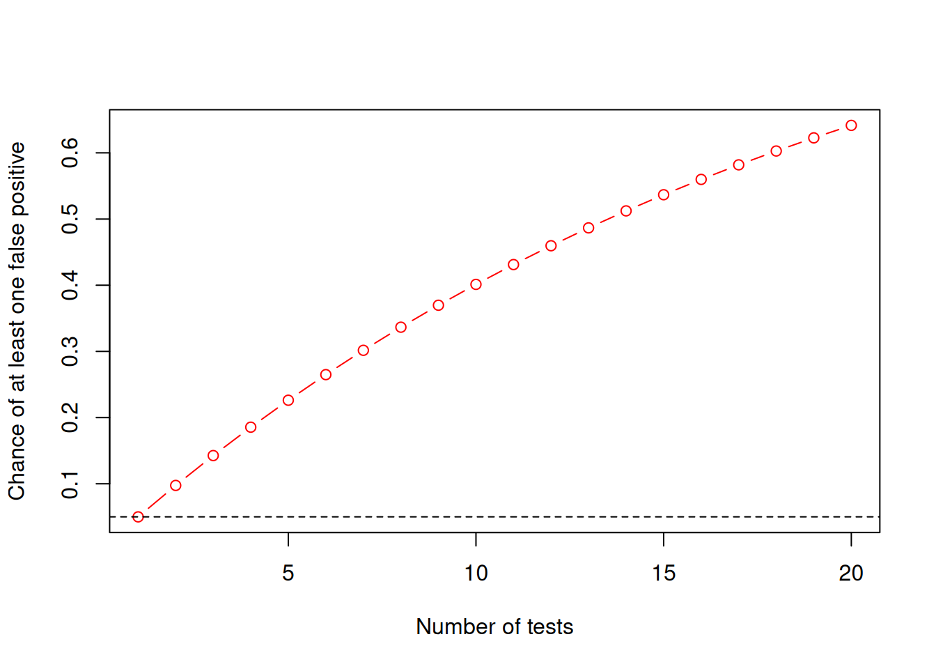
9) How big? Eta-squared
ss <- anova(m_var)$"Sum Sq"
ss[1] / sum(ss)              # eta-squared: share of variation explained by variety
[1] 0.6333067summary(m_var)$r.squared # the same, with one factor[1] 0.6333067Part C. Two factors
10) Additive: one drought effect for every variety
ggplot(trial, aes(variety, yield, colour = water)) +
  geom_point(position = position_jitterdodge(jitter.width = 0.15, dodge.width = 0.6)) +
  labs(x = NULL, y = "Yield (t/ha)") +
  theme_classic()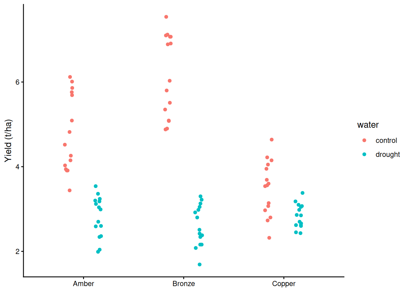
m_add <- lm(yield ~ variety + water, data = trial)
round(coef(summary(m_add)), 3)
Estimate Std. Error t value Pr(>|t|)
(Intercept) 4.819 0.190 25.364 0.000
varietyBronze 0.589 0.233 2.533 0.013
varietyCopper -0.627 0.233 -2.696 0.008
waterdrought -2.051 0.190 -10.796 0.00011) Interaction: each variety gets its own drought effect
m_int <- lm(yield ~ variety * water, data = trial)
round(coef(summary(m_int)), 3)
Estimate Std. Error t value Pr(>|t|)
(Intercept) 4.767 0.175 27.291 0
varietyBronze 1.389 0.247 5.621 0
varietyCopper -1.272 0.247 -5.149 0
waterdrought -1.948 0.247 -7.885 0
varietyBronze:waterdrought -1.599 0.349 -4.576 0
varietyCopper:waterdrought 1.289 0.349 3.690 0anova(m_int) # test the interaction row firstAnalysis of Variance Table
Response: yield
Df Sum Sq Mean Sq F value Pr(>F)
variety 2 22.211 11.106 24.263 4.820e-09 ***
water 1 94.659 94.659 206.807 < 2.2e-16 ***
variety:water 2 31.397 15.698 34.297 1.292e-11 ***
Residuals 84 38.448 0.458
---
Signif. codes: 0 '***' 0.001 '**' 0.01 '*' 0.05 '.' 0.1 ' ' 1Demo: a cell mean from the coefficients
b <- coef(m_int)
b["(Intercept)"] + b["varietyCopper"] + b["waterdrought"] + b["varietyCopper:waterdrought"]   # Copper, drought
(Intercept)
2.836667 Demo: a cell mean from the coefficients
mean(trial$yield[trial$variety == "Copper" & trial$water == "drought"])[1] 2.836667# interaction plot: predicted means, one line per variety
g <- expand.grid(variety = c("Amber", "Bronze", "Copper"), water = c("control", "drought"))
g$additive <- predict(m_add, g)
g$interaction <- predict(m_int, g)
ggplot(g, aes(water, interaction, colour = variety, group = variety)) +
geom_line(linewidth = 1.2) + geom_point(size = 3) +
labs(x = NULL, y = "Predicted yield (t/ha)") +
theme_classic()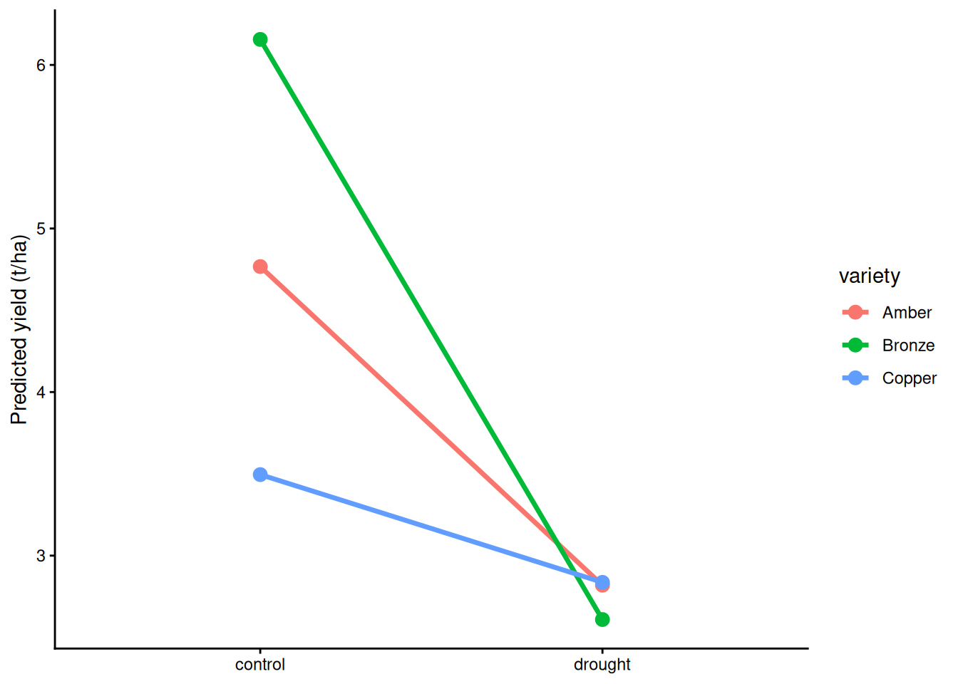
11b) summary() vs anova(): what is an “effect”?
Every row of summary() is one comparison between two cells. Every row of anova() is a whole term. With an interaction in the model, the “main effect” coefficients are effects at the reference level of the other factor: varietyCopper is Copper vs Amber under control only, and waterdrought is the drought effect in Amber only.
round(coef(summary(m_int)), 3)[, c(1, 4)] # single comparisons Estimate Pr(>|t|)
(Intercept) 4.767 0
varietyBronze 1.389 0
varietyCopper -1.272 0
waterdrought -1.948 0
varietyBronze:waterdrought -1.599 0
varietyCopper:waterdrought 1.289 0anova(m_int) # whole termsAnalysis of Variance Table
Response: yield
Df Sum Sq Mean Sq F value Pr(>F)
variety 2 22.211 11.106 24.263 4.820e-09 ***
water 1 94.659 94.659 206.807 < 2.2e-16 ***
variety:water 2 31.397 15.698 34.297 1.292e-11 ***
Residuals 84 38.448 0.458
---
Signif. codes: 0 '***' 0.001 '**' 0.01 '*' 0.05 '.' 0.1 ' ' 1Change the reference level: the coefficient changes (even its sign); the ANOVA table does not.
trial2$water <- factor(trial$water, levels = c("drought", "control"))
m_int2 <- lm(yield ~ variety * water, data = trial2)
round(coef(summary(m_int))["varietyCopper", ], 3)    # Copper - Amber, under control
Estimate Std. Error t value Pr(>|t|)
-1.272 0.247 -5.149 0.000 round(coef(summary(m_int2))["varietyCopper", ], 3) # Copper - Amber, under drought Estimate Std. Error t value Pr(>|t|)
0.017 0.247 0.070 0.944 anova(m_int)["variety", "Pr(>F)"][1] 4.81955e-09anova(m_int2)["variety", "Pr(>F)"] # identical[1] 4.81955e-09The anova() variety row is variety averaged over water. With a real interaction, that average can hide the story (emmeans warns you):
emmeans::emmeans(m_int, ~ variety) # averaged over water variety emmean SE df lower.CL upper.CL
Amber 3.79 0.124 84 3.55 4.04
Bronze 4.38 0.124 84 4.14 4.63
Copper 3.17 0.124 84 2.92 3.41
Results are averaged over the levels of: water
Confidence level used: 0.95 12) The effect within each variety: emmeans
library(emmeans)
emmeans(m_int, ~ water | variety)          # model-predicted means with CIs
variety = Amber:
water emmean SE df lower.CL upper.CL
control 4.77 0.175 84 4.42 5.11
drought 2.82 0.175 84 2.47 3.17
variety = Bronze:
water emmean SE df lower.CL upper.CL
control 6.16 0.175 84 5.81 6.50
drought 2.61 0.175 84 2.26 2.96
variety = Copper:
water emmean SE df lower.CL upper.CL
control 3.50 0.175 84 3.15 3.84
drought 2.84 0.175 84 2.49 3.18
Confidence level used: 0.95 pairs(emmeans(m_int, ~ water | variety)) # the drought effect in each varietyvariety = Amber:
contrast estimate SE df t.ratio p.value
control - drought 1.948 0.247 84 7.885 <0.0001
variety = Bronze:
contrast estimate SE df t.ratio p.value
control - drought 3.547 0.247 84 14.357 <0.0001
variety = Copper:
contrast estimate SE df t.ratio p.value
control - drought 0.659 0.247 84 2.666 0.009213) A second factor removes noise
anova(lm(yield ~ variety, data = trial)) # drought left in the residualsAnalysis of Variance Table
Response: yield
Df Sum Sq Mean Sq F value Pr(>F)
variety 2 22.211 11.1057 5.8734 0.004049 **
Residuals 87 164.504 1.8908
---
Signif. codes: 0 '***' 0.001 '**' 0.01 '*' 0.05 '.' 0.1 ' ' 1anova(m_add) # drought accounted forAnalysis of Variance Table
Response: yield
Df Sum Sq Mean Sq F value Pr(>F)
variety 2 22.211 11.106 13.675 6.974e-06 ***
water 1 94.659 94.659 116.553 < 2.2e-16 ***
Residuals 86 69.845 0.812
---
Signif. codes: 0 '***' 0.001 '**' 0.01 '*' 0.05 '.' 0.1 ' ' 114) Unequal group sizes: order matters
unbal <- trial[-(1:20), ]        # lose 20 plots
table(unbal$variety, unbal$water)
         control drought
  Amber       13      12
  Bronze      12      13
Copper 9 11anova(lm(yield ~ variety + water, data = unbal)) # sequential (Type I)Analysis of Variance Table
Response: yield
Df Sum Sq Mean Sq F value Pr(>F)
variety 2 14.504 7.252 9.3521 0.0002655 ***
water 1 87.703 87.703 113.1032 6.015e-16 ***
Residuals 66 51.178 0.775
---
Signif. codes: 0 '***' 0.001 '**' 0.01 '*' 0.05 '.' 0.1 ' ' 1anova(lm(yield ~ water + variety, data = unbal)) # the other orderAnalysis of Variance Table
Response: yield
Df Sum Sq Mean Sq F value Pr(>F)
water 1 89.153 89.153 114.9727 4.257e-16 ***
variety 2 13.054 6.527 8.4174 0.0005545 ***
Residuals 66 51.178 0.775
---
Signif. codes: 0 '***' 0.001 '**' 0.01 '*' 0.05 '.' 0.1 ' ' 1library(car)
Anova(lm(yield ~ variety + water, data = unbal), type = 2) # each adjusted for the otherAnova Table (Type II tests)
Response: yield
Sum Sq Df F value Pr(>F)
variety 13.054 2 8.4174 0.0005545 ***
water 87.703 1 113.1032 6.015e-16 ***
Residuals 51.178 66
---
Signif. codes: 0 '***' 0.001 '**' 0.01 '*' 0.05 '.' 0.1 ' ' 114b) Type III, and the contrasts trap
Type III adjusts every term for every other term, the interaction included. With an interaction, variety has a different effect at each water level, so Type III has to test it somewhere. With R’s default contrasts, its “variety” row tests variety at the reference water level (like the summary() row), so the answer changes with the reference. With sum-to-zero contrasts it tests variety averaged over water. This happens in balanced data too: it comes from the interaction, not from unequal group sizes.
library(car)
Anova(m_int, type = 3)["variety", 3:4]    # control as reference: F = 58
F value Pr(>F)
variety 58.036 < 2.2e-16 ***
---
Signif. codes: 0 '***' 0.001 '**' 0.01 '*' 0.05 '.' 0.1 ' ' 1Anova(m_int2, type = 3)["variety", 3:4] # drought as reference: nothing F value Pr(>F)
variety 0.5248 0.5936options(contrasts = c("contr.sum", "contr.poly"))
m_sum <- lm(yield ~ variety * water, data = trial)
Anova(m_sum, type = 3) # sum-to-zero: variety averaged over waterAnova Table (Type III tests)
Response: yield
Sum Sq Df F value Pr(>F)
(Intercept) 1286.41 1 2810.497 < 2.2e-16 ***
variety 22.21 2 24.263 4.820e-09 ***
water 94.66 1 206.807 < 2.2e-16 ***
variety:water 31.40 2 34.297 1.292e-11 ***
Residuals 38.45 84
---
Signif. codes: 0 '***' 0.001 '**' 0.01 '*' 0.05 '.' 0.1 ' ' 1options(contrasts = c("contr.treatment", "contr.poly")) # back to the default
emmeans::joint_tests(m_int) # the same averaged tests, whatever the coding model term df1 df2 F.ratio p.value
variety 2 84 24.263 <0.0001
water 1 84 206.807 <0.0001
variety:water 2 84 34.297 <0.0001Demo: what the variety columns are under each coding
cells <- data.frame(variety = rep(c("Amber", "Bronze", "Copper"), 2), water = rep(c("control", "drought"), each = 3))
model.matrix(~ variety * water, cells)        # treatment: interaction columns are 0 for every control row
(Intercept) varietyBronze varietyCopper waterdrought
1 1 0 0 0
2 1 1 0 0
3 1 0 1 0
4 1 0 0 1
5 1 1 0 1
6 1 0 1 1
varietyBronze:waterdrought varietyCopper:waterdrought
1 0 0
2 0 0
3 0 0
4 0 0
5 1 0
6 0 1
attr(,"assign")
[1] 0 1 1 2 3 3
attr(,"contrasts")
attr(,"contrasts")$variety
[1] "contr.treatment"
attr(,"contrasts")$water
[1] "contr.treatment"Demo: what the variety columns are under each coding
options(contrasts = c("contr.sum", "contr.poly"))
model.matrix(~ variety * water, cells)        # sum-to-zero: +1/-1 in both water levels
(Intercept) variety1 variety2 water1 variety1:water1 variety2:water1
1 1 1 0 1 1 0
2 1 0 1 1 0 1
3 1 -1 -1 1 -1 -1
4 1 1 0 -1 -1 0
5 1 0 1 -1 0 -1
6 1 -1 -1 -1 1 1
attr(,"assign")
[1] 0 1 1 2 3 3
attr(,"contrasts")
attr(,"contrasts")$variety
[1] "contr.sum"
attr(,"contrasts")$water
[1] "contr.sum"Demo: what the variety columns are under each coding
options(contrasts = c("contr.treatment", "contr.poly"))Which type? Balanced design: Types I, II, and III (with contr.sum) agree. Unbalanced: Type I only if the order means something; Type II when there is no interaction; Type III with contr.sum if you must test main effects alongside an interaction. If the interaction is real, report the effects within each level (emmeans) instead.
Part D. Groups and a slope together (ANCOVA)
15) Parallel lines
m_anc <- lm(yield ~ nitrogen + water, data = trial)
round(coef(summary(m_anc)), 4)   # intercept = control at 0 kg N
Estimate Std. Error t value Pr(>|t|)
(Intercept) 3.6962 0.1942 19.0350 0
nitrogen 0.0113 0.0015 7.2995 0
waterdrought -2.0491 0.1708 -11.9986 016) Different slopes
m_anc2 <- lm(yield ~ nitrogen * water, data = trial)
round(coef(summary(m_anc2)), 4)
Estimate Std. Error t value Pr(>|t|)
(Intercept) 3.1458 0.2113 14.8864 0.0000
nitrogen 0.0169 0.0018 9.1614 0.0000
waterdrought -0.7704 0.3160 -2.4382 0.0168
nitrogen:waterdrought -0.0130 0.0028 -4.6312 0.0000# nitrogen slope under drought: nitrogen + nitrogen:waterdrought
coef(m_anc2)["nitrogen"] + coef(m_anc2)["nitrogen:waterdrought"] nitrogen
0.003868891 With the interaction in, waterdrought is the drought effect at 0 kg N. Centre nitrogen and it becomes the drought effect at the average rate:
trial$nitrogen_c <- trial$nitrogen - mean(trial$nitrogen)
m_anc3 <- lm(yield ~ nitrogen_c * water, data = trial)
round(coef(summary(m_anc3)), 4)
Estimate Std. Error t value Pr(>|t|)
(Intercept) 4.8047 0.1087 44.2171 0
nitrogen_c 0.0169 0.0018 9.1614 0
waterdrought -2.0493 0.1537 -13.3354 0
nitrogen_c:waterdrought -0.0130 0.0028 -4.6312 0# one fitted line per group
ggplot(trial, aes(nitrogen, yield, colour = water)) +
geom_point() +
geom_smooth(method = "lm", se = FALSE) + # separate slopes, like nitrogen * water
labs(x = "Nitrogen (kg N/ha)", y = "Yield (t/ha)") +
theme_classic()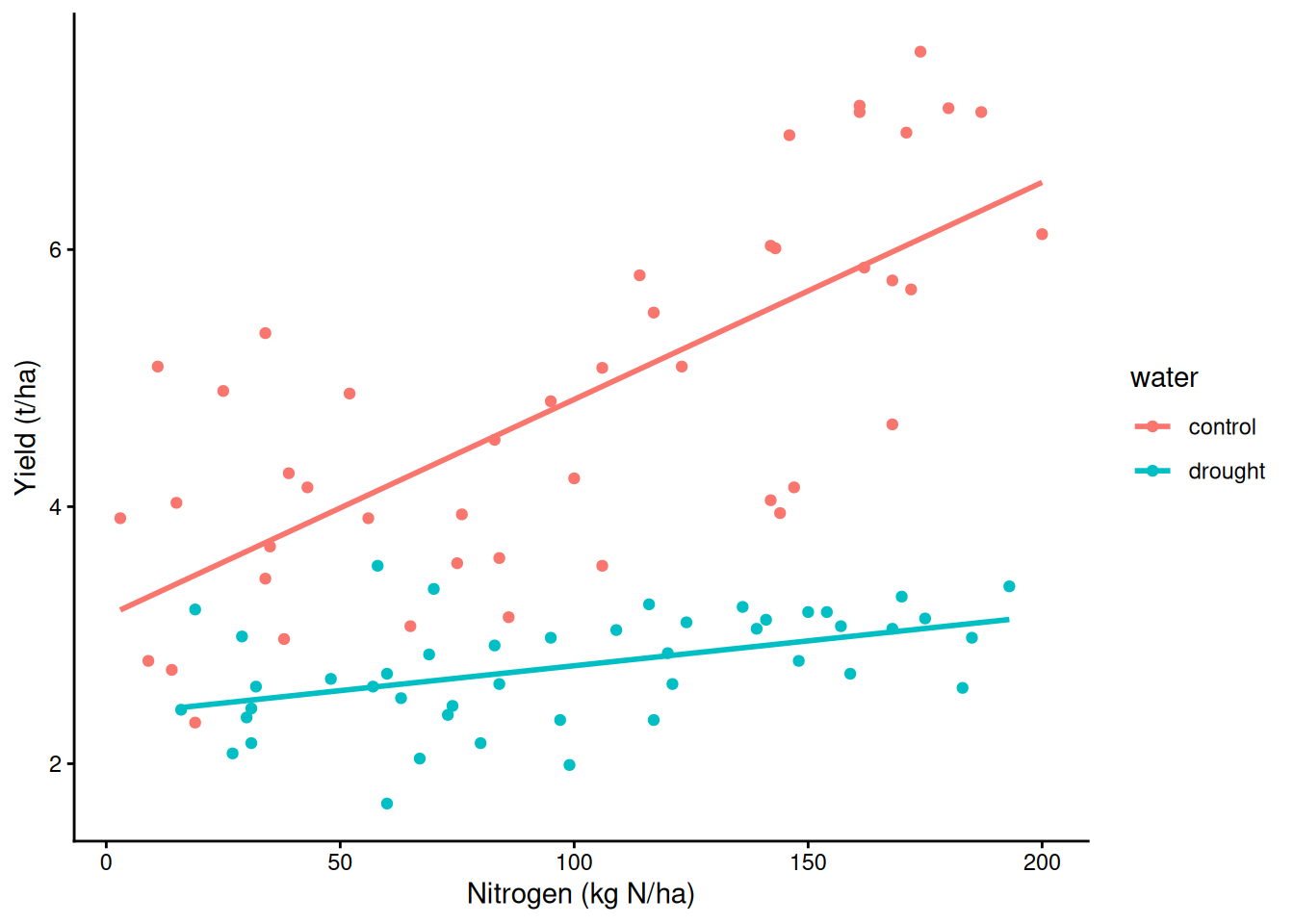
16b) Two numeric predictors: the main-effect t-test is the slope at 0
With nitrogen * water, the nitrogen coefficient is the nitrogen slope where water = 0. Here no plot is that dry, and the coefficient looks like nothing while anova() calls nitrogen one of the strongest terms.
Demo: simulate an irrigation x nitrogen trial
set.seed(47)
irrig <- data.frame(nitrogen = round(runif(60, 0, 200)),
                    water = round(runif(60, 15, 45)))   # mm/week
irrig$yield <- round(2 + 0.04 * irrig$water +
  0.0004 * irrig$nitrogen * irrig$water + rnorm(60, 0, 0.6), 2)
m_nw <- lm(yield ~ nitrogen * water, data = irrig)
round(coef(summary(m_nw)), 4) # nitrogen: the slope at water = 0 Estimate Std. Error t value Pr(>|t|)
(Intercept) 2.4875 0.4687 5.3075 0.0000
nitrogen -0.0021 0.0044 -0.4826 0.6313
water 0.0222 0.0158 1.4020 0.1664
nitrogen:water 0.0006 0.0002 3.6356 0.0006anova(m_nw) # nitrogen: a whole term, entered firstAnalysis of Variance Table
Response: yield
Df Sum Sq Mean Sq F value Pr(>F)
nitrogen 1 36.631 36.631 124.773 7.122e-16 ***
water 1 21.907 21.907 74.621 6.966e-12 ***
nitrogen:water 1 3.880 3.880 13.217 0.0006043 ***
Residuals 56 16.440 0.294
---
Signif. codes: 0 '***' 0.001 '**' 0.01 '*' 0.05 '.' 0.1 ' ' 1# centre both, refit: same fit, same interaction; main effects now at the means
irrig$nitrogen_c <- irrig$nitrogen - mean(irrig$nitrogen)
irrig$water_c <- irrig$water - mean(irrig$water)
m_nwc <- lm(yield ~ nitrogen_c * water_c, data = irrig)
round(coef(summary(m_nwc)), 4) Estimate Std. Error t value Pr(>|t|)
(Intercept) 4.4423 0.0700 63.5072 0e+00
nitrogen_c 0.0140 0.0012 11.5990 0e+00
water_c 0.0735 0.0083 8.8964 0e+00
nitrogen_c:water_c 0.0006 0.0002 3.6356 6e-04c(summary(m_nw)$r.squared, summary(m_nwc)$r.squared) # identical[1] 0.7915204 0.7915204Demo: the nitrogen slope at every water level, and how the tests line up
b <- coef(m_nw); V <- vcov(m_nw)
w <- seq(0, 50, by = 0.5)
slope <- b["nitrogen"] + b["nitrogen:water"] * w
se <- sqrt(V["nitrogen", "nitrogen"] + w^2 * V["nitrogen:water", "nitrogen:water"] + 2 * w * V["nitrogen", "nitrogen:water"])
plot(w, slope, type = "l", lwd = 2, col = "blue", ylim = range(slope - 2 * se, slope + 2 * se),
     xlab = "Water (mm/week)", ylab = "Nitrogen slope (t/ha per kg N)")
lines(w, slope - 2 * se, lty = 3, col = "blue"); lines(w, slope + 2 * se, lty = 3, col = "blue")
abline(h = 0, lty = 2); abline(v = range(irrig$water), col = "grey")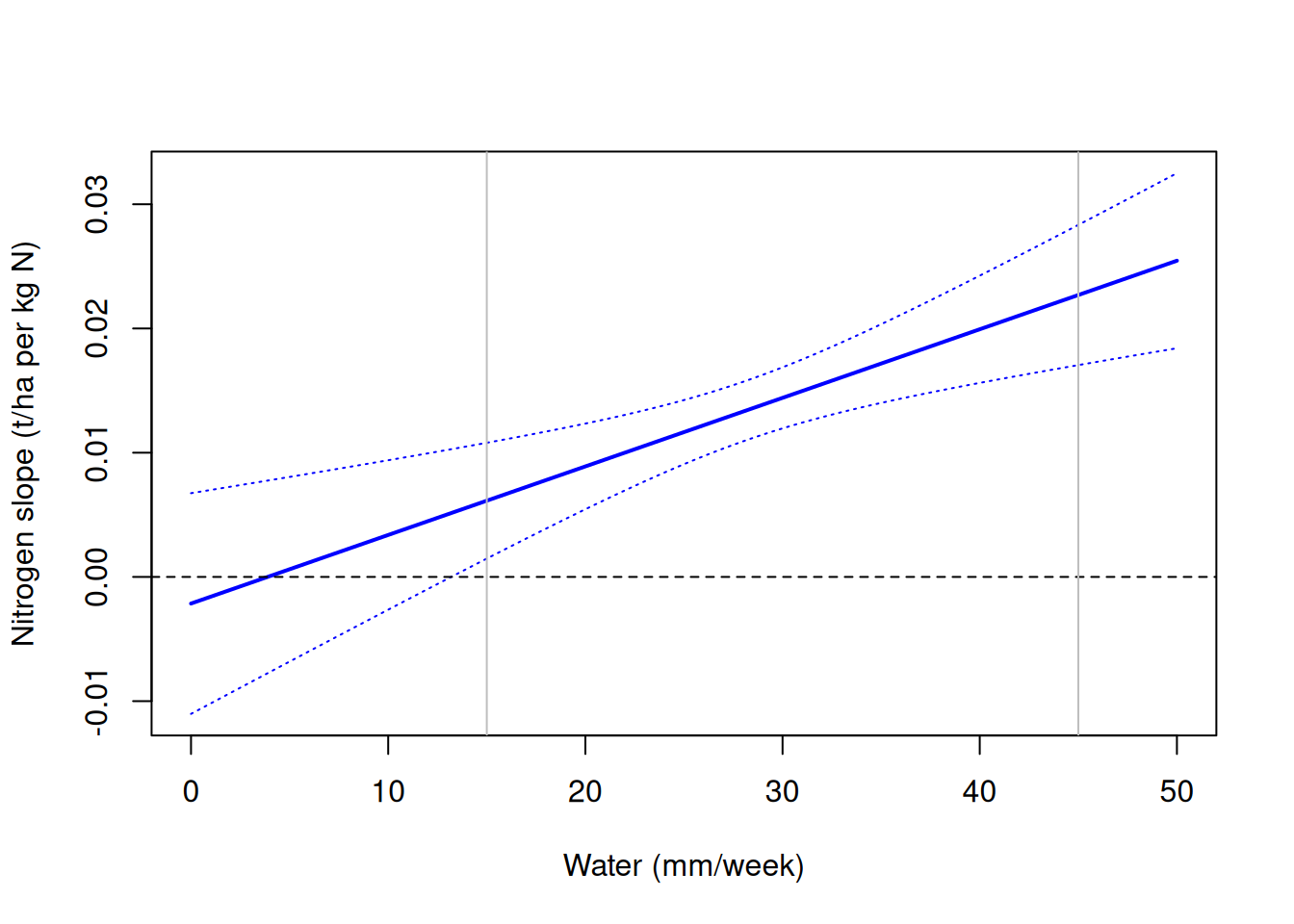
Demo: the nitrogen slope at every water level, and how the tests line up
# centred t^2 = Type III F; Type I and II test nitrogen without the interaction
coef(summary(m_nwc))["nitrogen_c", "t value"]^2
[1] 134.5374Demo: the nitrogen slope at every water level, and how the tests line up
library(car)
Anova(m_nwc, type = 3)["nitrogen_c", "F value"]
[1] 134.5374Demo: the nitrogen slope at every water level, and how the tests line up
Anova(m_nw, type = 2)["nitrogen", "F value"][1] 125.3709Demo: the nitrogen slope at every water level, and how the tests line up
Anova(m_nw, type = 3)["nitrogen", "F value"] # uncentred Type III: the same at-zero test[1] 0.2328861Part E. Yes/no responses: logistic regression
17) A straight line fails
m_lin <- lm(rust ~ nitrogen + variety + water, data = trial)
range(fitted(m_lin))                          # fitted "probabilities" for the real plots
[1] -0.107848 1.151009sum(fitted(m_lin) < 0 | fitted(m_lin) > 1) # how many are impossible[1] 1418) Probability, odds, log-odds
p <- c(0.2, 0.5, 0.8, 0.99)
odds <- p / (1 - p)
cbind(p, odds, log_odds = log(odds))
p odds log_odds
[1,] 0.20 0.25 -1.386294
[2,] 0.50 1.00 0.000000
[3,] 0.80 4.00 1.386294
[4,] 0.99 99.00 4.595120qlogis(0.8) # probability -> log-odds[1] 1.386294plogis(1.39) # log-odds -> probability[1] 0.8005922Demo: the logit curve and the S-curve
par(mfrow = c(1, 2))
curve(qlogis(x), 0.005, 0.995, xlab = "Probability", ylab = "Log-odds", col = "blue", lwd = 2)
curve(plogis(x), -6, 6, xlab = "Log-odds", ylab = "Probability", col = "red", lwd = 2)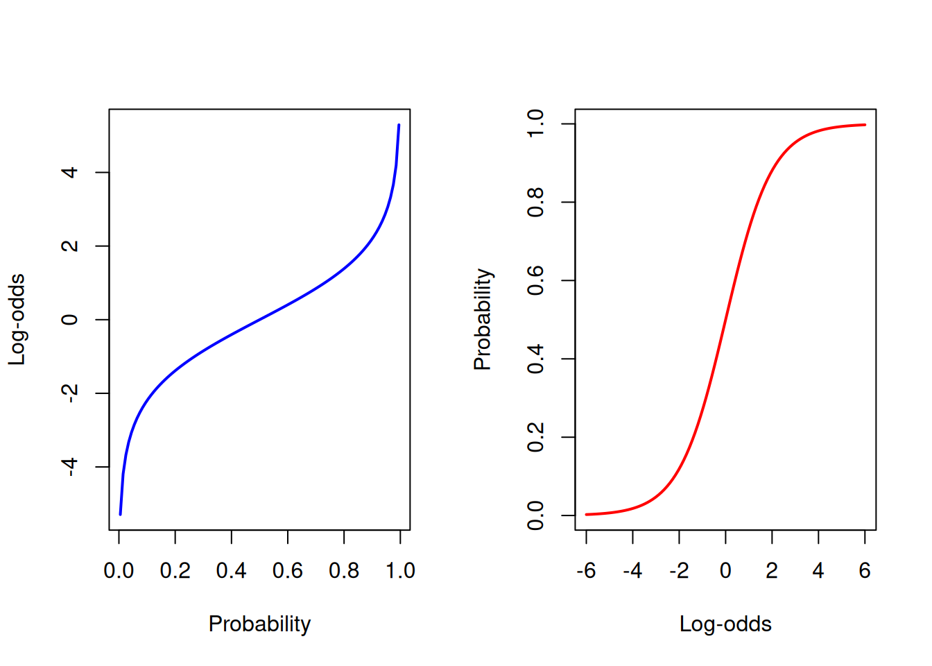
Demo: the logit curve and the S-curve
par(mfrow = c(1, 1))19) A group as the predictor
table(trial$rust, trial$water)
    control drought
  0      15      34
  1      30      11
m_rw <- glm(rust ~ water, family = binomial, data = trial)
round(coef(summary(m_rw)), 3) # log-odds scale Estimate Std. Error z value Pr(>|z|)
(Intercept) 0.693 0.316 2.192 0.028
waterdrought -1.822 0.469 -3.881 0.000plogis(coef(m_rw)[1]) # P(rust), control(Intercept)
0.6666667 plogis(sum(coef(m_rw))) # P(rust), drought[1] 0.2444444prop.table(table(trial$rust, trial$water), 2)
      control   drought
  0 0.3333333 0.7555556
1 0.6666667 0.2444444exp(coef(m_rw)) # odds ratio for drought (Intercept) waterdrought
2.0000000 0.1617647 exp(confint(m_rw)) 2.5 % 97.5 %
(Intercept) 1.09389806 3.8177252
waterdrought 0.06218335 0.3951711# the older tools for a 2 x 2 table ask the same question
fisher.test(table(trial$water, trial$rust))
    Fisher's Exact Test for Count Data

data:  table(trial$water, trial$rust)
p-value = 0.0001124
alternative hypothesis: true odds ratio is not equal to 1
95 percent confidence interval:
 0.05787788 0.44303705
sample estimates:
odds ratio
0.1655375 chisq.test(table(trial$water, trial$rust))
    Pearson's Chi-squared test with Yates' continuity correction

data:  table(trial$water, trial$rust)
X-squared = 14.515, df = 1, p-value = 0.0001391
20) A continuous predictor
m_rn <- glm(rust ~ nitrogen, family = binomial, data = trial)
round(coef(summary(m_rn)), 4)
Estimate Std. Error z value Pr(>|z|)
(Intercept) -1.7047 0.5046 -3.3784 7e-04
nitrogen 0.0152 0.0044 3.4533 6e-04exp(10 * coef(m_rn)["nitrogen"]) # odds ratio per 10 kg Nnitrogen
1.164638 -coef(m_rn)[1] / coef(m_rn)[2] # nitrogen where P(rust) = 0.5(Intercept)
111.8488 # plot the fitted curve: predict probabilities over a grid
grid <- data.frame(nitrogen = 0:200)
grid$p <- predict(m_rn, newdata = grid, type = "response")
plot(trial$nitrogen, jitter(trial$rust, 0.1), xlab = "Nitrogen (kg N/ha)", ylab = "Rust (0/1)")
lines(grid$nitrogen, grid$p, col = "red", lwd = 2)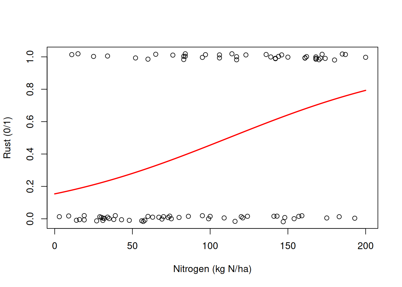
21) predict(): log-odds or probability
new <- data.frame(nitrogen = c(50, 100, 150))
predict(m_rn, newdata = new)                     # log-odds (the default)
1 2 3
-0.9426418 -0.1805881 0.5814655 predict(m_rn, newdata = new, type = "response") # probability 1 2 3
0.2803670 0.4549753 0.6414046 head(fitted(m_rn)) # fitted() is always probability 1 2 3 4 5 6
0.1954285 0.2338857 0.7385986 0.3220192 0.5196175 0.1837236 22) How often is it right?
pred <- as.numeric(fitted(m_rn) > 0.5)
table(predicted = pred, observed = trial$rust)   # confusion matrix
observed
predicted 0 1
0 35 16
1 14 25mean(pred == trial$rust) # accuracy[1] 0.6666667mean(trial$rust == 0) # always guess "no rust": the baseline to beat[1] 0.544444423) Several predictors
m_rall <- glm(rust ~ nitrogen + variety + water, family = binomial, data = trial)
round(coef(summary(m_rall)), 3)
Estimate Std. Error z value Pr(>|z|)
(Intercept) -1.598 0.718 -2.227 0.026
nitrogen 0.020 0.006 3.489 0.000
varietyBronze 2.231 0.768 2.904 0.004
varietyCopper 0.084 0.679 0.123 0.902
waterdrought -2.725 0.668 -4.078 0.000round(exp(coef(m_rall)), 2) # odds ratios, each holding the others fixed (Intercept) nitrogen varietyBronze varietyCopper waterdrought
0.20 1.02 9.31 1.09 0.07 24) Deviance
m_rall$null.deviance # intercept only[1] 124.0544deviance(m_rall) # with the predictors[1] 77.892121 - deviance(m_rall) / m_rall$null.deviance # McFadden's pseudo-R2[1] 0.3721134anova(m_rn, m_rall, test = "Chisq") # nested GLMs: likelihood-ratio testAnalysis of Deviance Table
Model 1: rust ~ nitrogen
Model 2: rust ~ nitrogen + variety + water
Resid. Df Resid. Dev Df Deviance Pr(>Chi)
1 88 110.327
2 85 77.892 3 32.435 4.238e-07 ***
---
Signif. codes: 0 '***' 0.001 '**' 0.01 '*' 0.05 '.' 0.1 ' ' 125) Counts out of a total: cbind(successes, failures)
Demo: simulate germination in 30 trays of 20 seeds
set.seed(3)
trays <- data.frame(temp = runif(30, 8, 30))
trays$germ <- rbinom(30, 20, plogis(-4 + 0.25 * trays$temp))
m_g <- glm(cbind(germ, 20 - germ) ~ temp, family = binomial, data = trays)
round(coef(summary(m_g)), 3) Estimate Std. Error z value Pr(>|z|)
(Intercept) -4.090 0.379 -10.784 0
temp 0.266 0.022 12.281 0exp(coef(m_g)["temp"]) # odds of germinating, per degree temp
1.305303 26) More than two categories: multinomial
library(nnet)
m_sp <- multinom(Species ~ Petal.Length + Petal.Width, data = iris, trace = FALSE)
table(predicted = predict(m_sp), observed = iris$Species)
observed
predicted setosa versicolor virginica
setosa 50 0 0
versicolor 0 47 3
virginica 0 3 47Part F. Counts: Poisson regression
27) Last week’s seed counts
Demo: simulate last week’s seed counts
set.seed(4)
size  <- runif(80, 1, 10)
seeds <- rpois(80, lambda = exp(-1 + 0.35 * size))
pods  <- data.frame(size, seeds)
m_pod <- glm(seeds ~ size, family = poisson, data = pods)
round(coef(summary(m_pod)), 3) # log scale Estimate Std. Error z value Pr(>|z|)
(Intercept) -1.222 0.238 -5.138 0
size 0.377 0.029 13.009 0exp(coef(m_pod)) # rate ratio: x 1.46 seeds per unit of size(Intercept) size
0.294559 1.457612 # the Poisson curve vs last week's straight line
grid <- data.frame(size = seq(0, 10, by = 0.1))
plot(pods$size, pods$seeds, xlab = "Plant size", ylab = "Seeds per plant")
abline(lm(seeds ~ size, data = pods), lty = 2)
lines(grid$size, predict(m_pod, newdata = grid, type = "response"), col = "red", lwd = 2)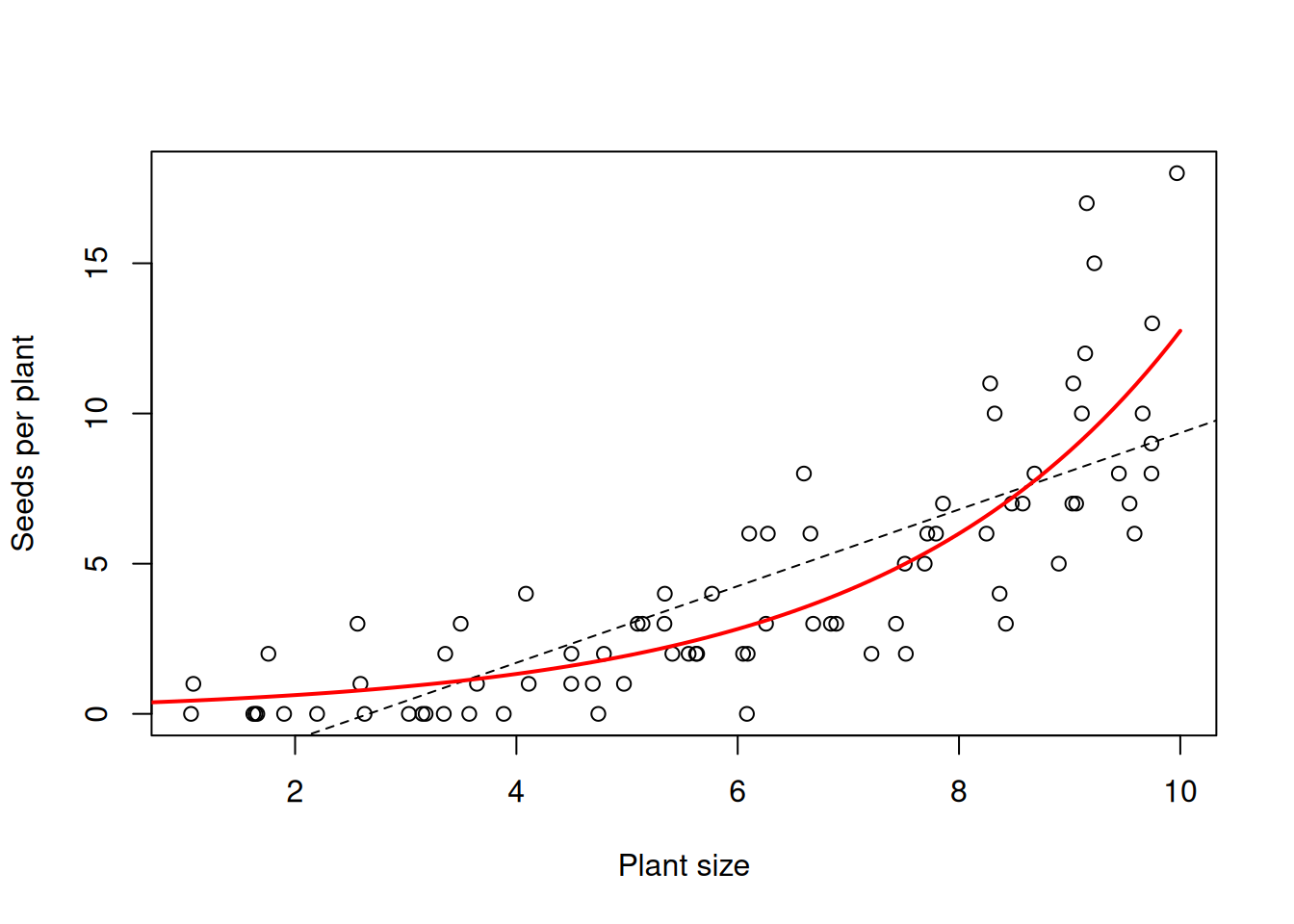
28) Aphids, and overdispersion
m_aph <- glm(aphids ~ nitrogen, family = poisson, data = trial)
round(coef(summary(m_aph)), 4)
Estimate Std. Error z value Pr(>|z|)
(Intercept) 1.1307 0.0914 12.3743 0
nitrogen 0.0101 0.0007 15.1468 0deviance(m_pod) / df.residual(m_pod) # about 1: fine[1] 1.187493deviance(m_aph) / df.residual(m_aph) # about 6: overdispersed[1] 5.6965629) Fix: negative binomial (or quasipoisson)
library(MASS)
m_nb <- glm.nb(aphids ~ nitrogen, data = trial)
round(coef(summary(m_nb)), 4)   # same slope, honest SE
Estimate Std. Error z value Pr(>|z|)
(Intercept) 1.1020 0.1872 5.8861 0
nitrogen 0.0103 0.0016 6.4848 0m_qp <- glm(aphids ~ nitrogen, family = quasipoisson, data = trial)
round(coef(summary(m_qp)), 4) # same slope as Poisson, SE scaled by the dispersion Estimate Std. Error t value Pr(>|t|)
(Intercept) 1.1307 0.2192 5.1584 0
nitrogen 0.0101 0.0016 6.3142 0Part G. Reporting
30) Odds ratios and rate ratios with CIs, on a sensible step
exp(10 * coef(m_rn)["nitrogen"])nitrogen
1.164638 exp(10 * confint(m_rn)["nitrogen", ]) 2.5 % 97.5 %
1.072029 1.276117 # "The odds of rust increased with nitrogen (odds ratio 1.16 per 10 kg N,
# 95% CI 1.07 to 1.28; z = 3.5, p < 0.001; logistic regression, n = 90)."
exp(10 * coef(m_nb)["nitrogen"])nitrogen
1.108852 exp(10 * confint(m_nb)["nitrogen", ]) 2.5 % 97.5 %
1.074744 1.144430 # "Aphid counts increased with nitrogen (rate ratio 1.11 per 10 kg N,
# 95% CI 1.07 to 1.14; negative binomial GLM, n = 90)."Part H. Bonus: mixed effect models
31) Plots grouped on farms
112 plots on 12 farms (2 to 25 plots each). Nitrogen raises yield everywhere, each farm has its own baseline, and cover crops (chosen per farm) do nothing.
Demo: simulate 112 plots on 12 farms
set.seed(181)
nj <- c(2, 2, 3, 4, 5, 6, 8, 10, 12, 15, 20, 25)   # plots per farm
ids <- sprintf("farm%02d", 1:12)
cover_j <- setNames(rep(c("no", "yes"), 6)[sample(12)], ids)
u <- setNames(rnorm(12, 0, 0.8), ids)              # each farm: its own baseline
farm <- rep(ids, nj)
nitrogen <- round(runif(112, 0, 200))
yield <- round(3.5 + 0.012 * nitrogen + u[farm] + rnorm(112, 0, 1), 2)
farms <- data.frame(farm, cover = unname(cover_j[farm]), nitrogen, yield)head(farms, 4) farm cover nitrogen yield
1 farm01 no 24 2.88
2 farm01 no 31 4.18
3 farm02 yes 145 4.64
4 farm02 yes 2 2.85table(farms$farm)
farm01 farm02 farm03 farm04 farm05 farm06 farm07 farm08 farm09 farm10 farm11
     2      2      3      4      5      6      8     10     12     15     20
farm12
    25
32) Farm as fixed vs random
# install.packages("lme4")
library(lme4)
m_fixed <- lm(yield ~ nitrogen + farm, data = farms)          # 12 free intercepts
m_mixed <- lmer(yield ~ nitrogen + (1 | farm), data = farms)  # farms drawn from N(0, sd_farm^2)
VarCorr(m_mixed)                       # two variance components
Groups Name Std.Dev.
farm (Intercept) 0.75921
Residual 1.01835 round(coef(summary(m_mixed)), 4) # fixed effects (no p-values: see lmerTest) Estimate Std. Error t value
(Intercept) 3.3377 0.3001 11.1219
nitrogen 0.0113 0.0017 6.6802round(coef(summary(m_fixed))["nitrogen", ], 4) Estimate Std. Error t value Pr(>|t|)
0.0115 0.0017 6.6110 0.0000 33) Shrinkage: small farms borrow strength
Demo: farm effects, fixed vs random
ids <- sort(unique(farms$farm))
fixed  <- c(0, coef(m_fixed)[paste0("farm", ids[-1])]) + coef(m_fixed)[1] - fixef(m_mixed)[1]
random <- ranef(m_mixed)$farm[ids, 1]
n <- as.numeric(table(farms$farm)[ids])
plot(1:12, fixed, ylim = range(c(fixed, random)), xaxt = "n", xlab = "", ylab = "Farm effect (t/ha)")
axis(1, at = 1:12, labels = paste0("n=", n), cex.axis = 0.7)
points(1:12, random, pch = 16, col = "purple")
arrows(1:12, fixed, 1:12, random, length = 0.05, col = "purple")
abline(h = 0, lty = 2)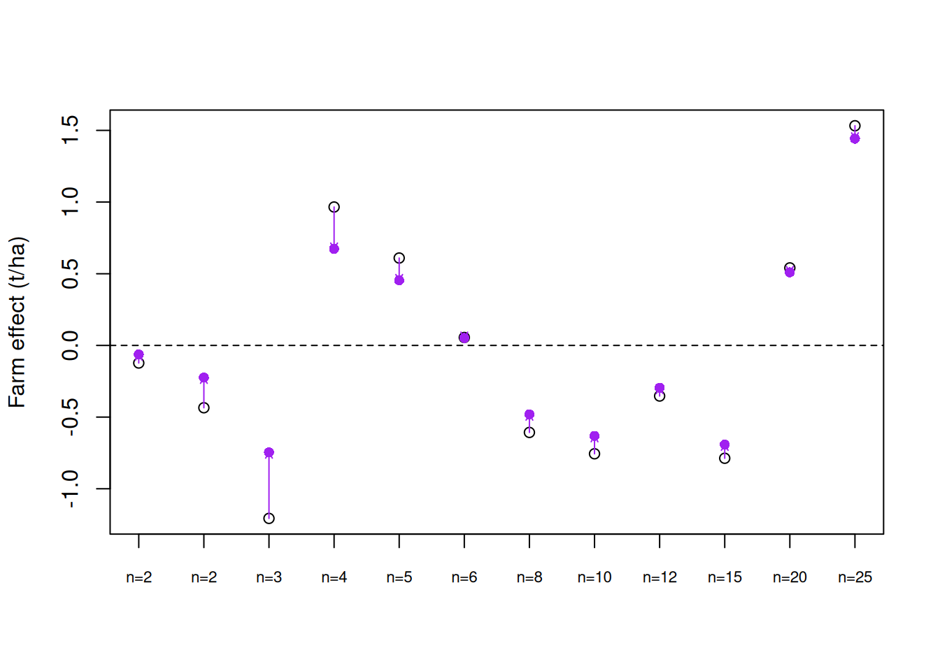
Demo: farm effects, fixed vs random
# the weight each farm keeps on its own estimate
sd_farm <- attr(VarCorr(m_mixed)$farm, "stddev"); s <- sigma(m_mixed)
round(sd_farm^2 / (sd_farm^2 + s^2 / n), 2)
[1] 0.53 0.53 0.63 0.69 0.74 0.77 0.82 0.85 0.87 0.89 0.92 0.9334) Why it matters: a treatment chosen per farm
round(coef(summary(lm(yield ~ nitrogen + cover, data = farms)))["coveryes", ], 4) # plots as independent: wrong Estimate Std. Error t value Pr(>|t|)
1.0139 0.2398 4.2289 0.0000 m_mixed2 <- lmer(yield ~ nitrogen + cover + (1 | farm), data = farms)
round(coef(summary(m_mixed2))["coveryes", ], 4) # farm in the model: honest Estimate Std. Error t value
0.2380 0.5142 0.4627 # checks: residuals as for lm(), and the farm effects should look normal
plot(m_mixed)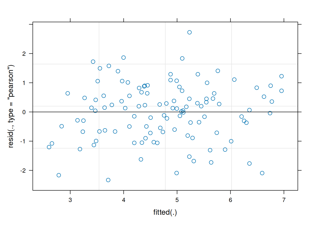
qqnorm(ranef(m_mixed)$farm[, 1]); qqline(ranef(m_mixed)$farm[, 1])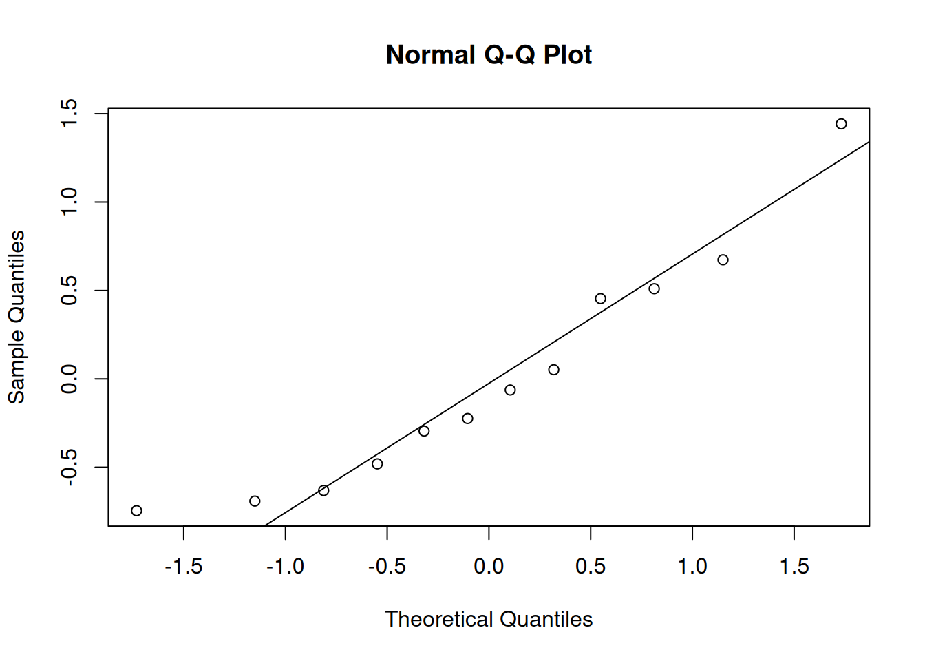
# the same for yes/no or counts: glmer(rust ~ nitrogen + (1 | block), family = binomial, data = ...)